使用Julia调用Sac并做图_non-original
过渡循规蹈矩,只会在既有的泥潭中越陷越深。就像写文章一样,如果总是想一气呵成或是一蹴而就如行云流水般写就,那结局必定是寸步难行,特别是对于我这样的新手难说更是如此。因此,我可以尝试老师说的方式,文章的结论部分不要一次写完,每一次写一点。用在这种学习笔记中便是:不能总想着一次就把第一部分完成,然后开始第二部分,可以先把“菜”下锅,等需要放什么的时候再来。
非原创
一、Julia基本操作及快捷键
Ctrl+? ,出现help?>,寻求帮助
],英文模式下输入,进入Pkg模式,我不太了解,尝试两次后的初步感觉是,它可以通过以给定链接的方式下载库并安装。
例如,进入Pkg模式后,添加模块的命令格式应为:
1 | pkg>add url |
例如:
1 | pkg>add https://github.com/anowacki/SeisRequests.jl |
当需要从Pkg模式下退出时,直接使用Backspace按键即可。
二、SeisRequests
准备工作
1.安装SAC.jl,可能需要编译SpecialFunctions
1 | pkg> add https://github.com/anowacki/SAC.jl |
2.安装SACPlot
1 | pkg> add https://github.com/anowacki/SACPlot.jl |
3.安装Plots
1 | julia> import Pkg; Pkg.add("Plots") |
使用说明
1.使用FDSN服务标准:
1 | FDSNEvent:查询事件 |
2.使用IRIS服务标准:
1 | IRISTimeSeries: 请求波形数据 |
3.REPL
待添加。。。。。。
4.所有请求由get_request函数发出,它会自动返回HTTP.message.Response,包含有服务器返回的信息。
示例
参考:https://github.com/anowacki/SeisRequests.jl
以获取2007年南威尔士地震数据为例:
1 | julia> using SeisRequests # 启动SeisRequests |
1 | julia> using Dates, SAC # `using Base.Dates` if still on Julia v1.0 |
结果:
三、关于SACPlot
1.plot1画单道
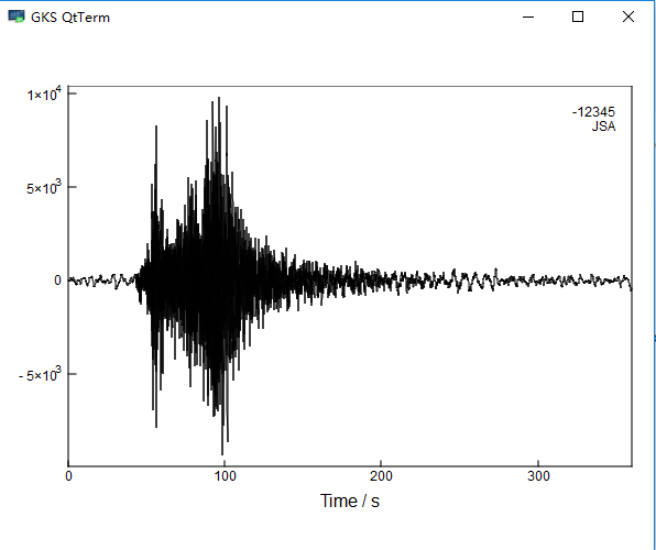
1 | julia> t=SAC.sample() |
结果:
2.plot1画多道
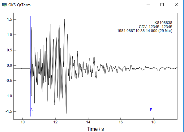
1 | julia> A = [SAC.sample() for i in 1:5] |> rtrend! |> taper! |
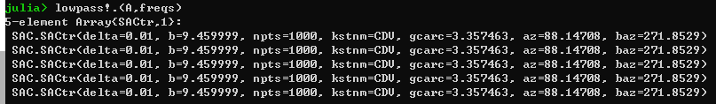
做低通滤波后:
最后一步成图:
1 | julia> pl(A) |
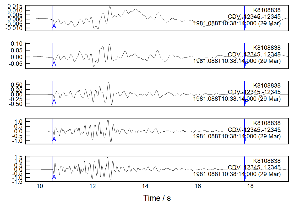
plotrs,添加标签
1
2
3
4
5julia> B = SAC.sample(:array); # Load sample data
julia> B = cut(B, :a, -30, :a, 30); # Cut traces
julia> import Pkg; Pkg.add("Plots"); # This allows us to call Plots directly below
julia> import Plots; Plots.default(size=(600,1000), margin=4Plots.mm) # Change the default figure size and margin
julia> plotrs(B, :a, qdp=false, label=:kstnm, xlabel="Time rel. PKIKP / s", ylabel="Distance / °")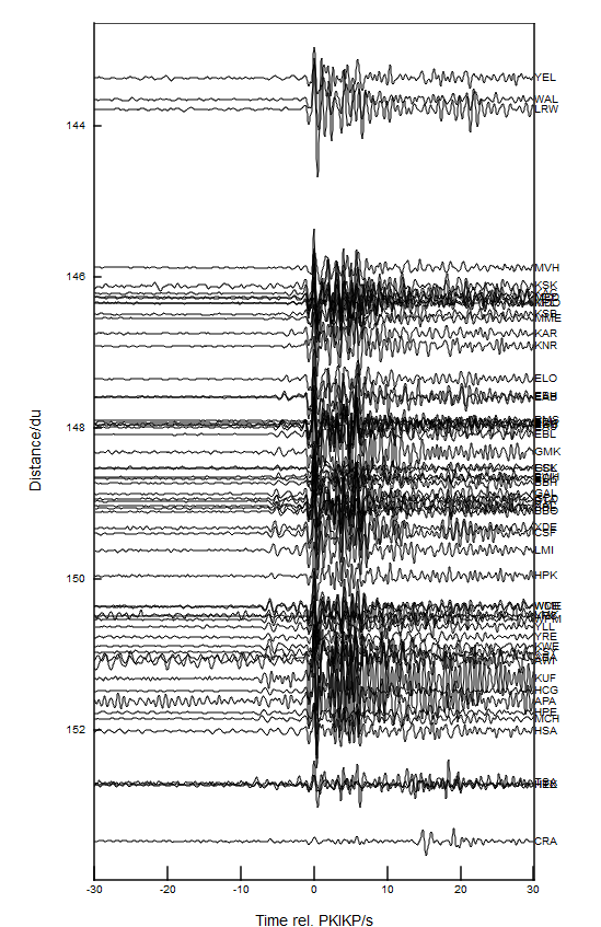
4.example plotrs
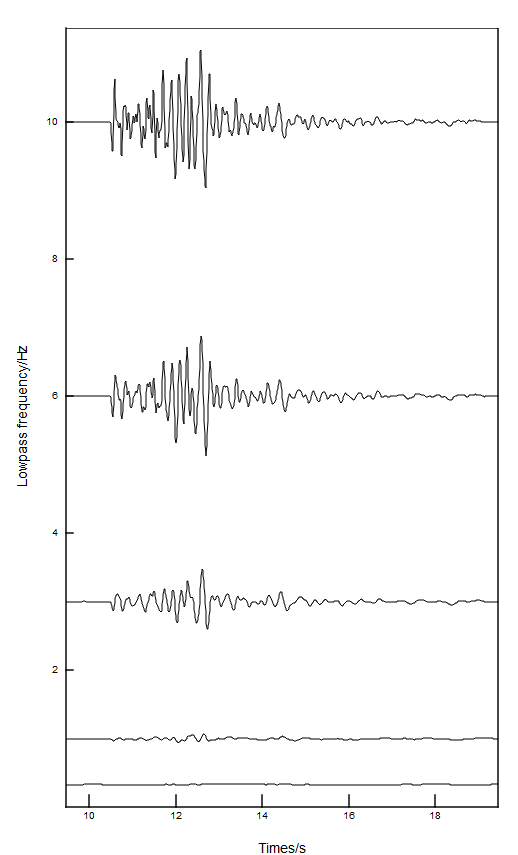
1 | julia> plotrs(A, y=:user0, xlabel="Time / s", ylabel="Lowpass frequency / Hz") |
参考:https://github.com/anowacki/SeisRequests.jl
修改历史:
- 2018-11-06,翻译初稿,后续想继续学习SAC在Julia中的使用,也借此绕开SAC对系统的限制,使用更快的Julia语言重新理解SAC。另外,必须清楚一条,程序语言的本质是解决问题,千万不要掉进去理解程序语言的每一个细节的这种“贪婪者”的陷阱。既然是在地震学中使用,那么只需要能解决问题便是王道。
Author: Crowboydoudou
Link: https://crowboydoudou.github.io/2018/11/19/使用Julia调用Sac并做图/
License: 知识共享署名-非商业性使用 4.0 国际许可协议